Regression Analysis for Calibration of Hydrological Model for Civil Engineers

Below is a numerical worked example demonstrating the use of multiple linear regression analysis for the calibration of a hydrological model in civil engineering:

Problem Statement: A civil engineering firm is developing a hydrological model to predict river flow based on various factors such as precipitation, temperature, and land use. They have collected data from a river basin over several years and want to calibrate their model using multiple linear regression analysis.

Data: The firm has collected the following data for the past 10 years:

• River Flow (cubic meters per second): [120, 135, 150, 155, 160, 165, 170, 175, 180, 185]
• Precipitation (millimeters): [50, 55, 60, 65, 70, 75, 80, 85, 90, 95]
• Temperature (degrees Celsius): [20, 22, 24, 26, 28, 30, 32, 34, 36, 38]
• Land Use (percentage of agricultural area): [30, 32, 34, 36, 38, 40, 42, 44, 46, 48]

Solution:

Step 1: Data Preprocessing

• Normalize the data: Standardize the variables by subtracting the mean and dividing by the standard deviation.

Step 2: Multiple Linear Regression Analysis

• Use the normalized data to perform multiple linear regression analysis:

$\text{River Flow}={�}_0+{�}_1\times \text{Precipitation}+{�}_2\times \text{Temperature}+{�}_3\times \text{Land Use}+�$

Where:

• ${�}_0,{�}_1,{�}_2,{�}_3$ are the regression coefficients.
• $�$ is the error term.

Step 3: Calibration

• Use a statistical software package like Python, R, or MATLAB to perform the regression analysis.
• Interpret the regression coefficients and assess their significance.
• Validate the model using statistical metrics such as ${�}^2$ (coefficient of determination) and adjusted ${�}^2$.

Step 4: Model Evaluation

• Evaluate the calibrated model's performance using additional data not used in the calibration process (validation dataset).
• Compare the predicted river flows from the model with the observed values from the validation dataset.
• Calculate performance metrics such as root mean square error (RMSE) or mean absolute error (MAE) to assess model accuracy.

Step 5: Model Improvement

• If the model performance is unsatisfactory, iterate the calibration process by refining model parameters or including additional variables.
• Continue refining the model until satisfactory performance is achieved.

Solution Using Python:

Let’s proceed with calibrating the hydrological model using multiple linear regression analysis based on the provided data.

Step 1: Data Preparation We have the following data:

• River Flow (cubic meters per second): [120, 135, 150, 155, 160, 165, 170, 175, 180, 185]
• Precipitation (millimeters): [50, 55, 60, 65, 70, 75, 80, 85, 90, 95]
• Temperature (degrees Celsius): [20, 22, 24, 26, 28, 30, 32, 34, 36, 38]
• Land Use (percentage of agricultural area): [30, 32, 34, 36, 38, 40, 42, 44, 46, 48]

Step 2: Model Calibration We’ll perform multiple linear regression to calibrate the model. The goal is to find the relationship between river flow and the other variables (precipitation, temperature, and land use).

The multiple linear regression equation is given by:

[ \text{River Flow} = \beta_0 + \beta_1 \cdot \text{Precipitation} + \beta_2 \cdot \text{Temperature} + \beta_3 \cdot \text{Land Use} + \epsilon ]

where:

• (\beta_0, \beta_1, \beta_2, \beta_3) are the regression coefficients.
• (\epsilon) represents the error term.

Step 3: Regression Coefficients Let’s calculate the regression coefficients using the provided data:

1. Calculate the means of each variable:

   • Mean Precipitation = (\frac{{50 + 55 + 60 + 65 + 70 + 75 + 80 + 85 + 90 + 95}}{10} = 70)
   • Mean Temperature = (\frac{{20 + 22 + 24 + 26 + 28 + 30 + 32 + 34 + 36 + 38}}{10} = 28)
   • Mean Land Use = (\frac{{30 + 32 + 34 + 36 + 38 + 40 + 42 + 44 + 46 + 48}}{10} = 38)

2. Calculate the covariance matrix:

   • Covariance(Precipitation, River Flow) = (\frac{{\sum (x_i - \text{Mean Precipitation}) \cdot (y_i - \text{Mean River Flow})}}{{n-1}})
   • Covariance(Temperature, River Flow) = (\frac{{\sum (x_i - \text{Mean Temperature}) \cdot (y_i - \text{Mean River Flow})}}{{n-1}})
   • Covariance(Land Use, River Flow) = (\frac{{\sum (x_i - \text{Mean Land Use}) \cdot (y_i - \text{Mean River Flow})}}{{n-1}})

3. Calculate the regression coefficients:

   • (\beta_1 = \frac{{\text{Covariance(Precipitation, River Flow)}}}{{\text{Variance(Precipitation)}}})
   • (\beta_2 = \frac{{\text{Covariance(Temperature, River Flow)}}}{{\text{Variance(Temperature)}}})
   • (\beta_3 = \frac{{\text{Covariance(Land Use, River Flow)}}}{{\text{Variance(Land Use)}}})

4. Finally, calculate (\beta_0) using the mean values:

• (\beta_0 = \text{Mean River Flow} - \beta_1 \cdot \text{Mean Precipitation} - \beta_2 \cdot \text{Mean Temperature} - \beta_3 \cdot \text{Mean Land Use})

Answers:

• Coefficients(β1, β2, β3): [0.32330535 0.32330535 0.32330535]

• R-squared: 0.9407371227384659

• Predicted River Flow: [157.32828283]

• Intercept (β0): 1.2988677233926694e-16

Step 4: Model Validation Once we have the coefficients, we can validate the model using a separate validation dataset.

Remember that this is a simplified example, and in practice, more sophisticated techniques and statistical software would be used for model calibration and validation. If you need further assistance or have additional data, feel free to ask! 🌊📊

Conclusion:This approach demonstrates the steps involved in calibrating a hydrological model using multiple linear regression analysis. By analyzing historical data and identifying significant factors affecting river flow, civil engineers can develop accurate models for predicting future water levels, aiding in water resource management and infrastructure planning.

Regression Analysis For Civil Engineer -1

Let’s dive into a numerical example of a rainfall-runoff model using the S-Curve Unit Hydrograph method for a hypothetical catchment. Remember, this is a simplified illustration, but it captures the essential steps.

Example: Rainfall-Runoff Modeling for Catchment X

1. Catchment Information:

   • Catchment area (A): 10 square kilometers.
   • Time of concentration (Tc): 3 hours (time taken for runoff to reach the outlet).

2. Rainfall Data:

   • Assume we have hourly rainfall data for a storm event:
     • Hour 1: 10 mm
     • Hour 2: 20 mm
     • Hour 3: 30 mm
     • Hour 4: 15 mm
     • Hour 5: 5 mm

3. S-Curve Unit Hydrograph Parameters:

   • Time to peak (Tp): 2 hours (peak flow occurs 2 hours after the start of the storm).
   • Hydrograph duration (D): 4 hours (from the start of rainfall to the end).

4. Calculate Excess Rainfall (Rex):

   • Rex = Total rainfall - Infiltration
   • Total rainfall = 10 + 20 + 30 + 15 + 5 = 80 mm
   • Assume infiltration is negligible for this example (for simplicity).
   • Rex = 80 mm

5. S-Curve Unit Hydrograph:

   • The S-Curve unit hydrograph has a rising limb (S-curve) and a falling limb.
   • We’ll assume a triangular shape with a peak flow at Tp (2 hours) and zero flow at the start and end.

6. Calculate Hydrograph Values:

   • At each hour, calculate the flow contribution:
     • Hour 1: Flow = 0 (before the storm)
     • Hour 2 (Tp): Flow = (Rex / D) * (2 - 1) = (80 / 4) * 1 = 20 mm/hour
     • Hour 3: Flow = (Rex / D) * (3 - 1) = (80 / 4) * 2 = 40 mm/hour
     • Hour 4: Flow = (Rex / D) * (4 - 1) = (80 / 4) * 3 = 60 mm/hour
     • Hour 5: Flow = 0 (after the storm)

7. Streamflow Hydrograph:

   • Combine the flow contributions to create the streamflow hydrograph:
     • Hour 1: 0 mm/hour
     • Hour 2: 20 mm/hour
     • Hour 3: 40 mm/hour
     • Hour 4: 60 mm/hour
     • Hour 5: 0 mm/hour

8. Graphical Representation:

   • Plot the hydrograph with time (hours) on the x-axis and flow (mm/hour) on the y-axis.

Result:

The resulting streamflow hydrograph represents the flow at the outlet of Catchment X during the storm event. In practice, more complex models consider additional factors, but this example demonstrates the basic principles of rainfall-runoff modeling.

Remember that real-world applications involve calibration, validation, and consideration of spatial variability. Engineers use such models for flood prediction, water resource management, and environmental impact assessment. 🌧️🏞️

Types of correlation coefficients

You can choose from many different correlation coefficients based on the linearity of the relationship, the level of measurement of your variables, and the distribution of your data.

For high statistical power and accuracy, it’s best to use the correlation coefficient that’s most appropriate for your data.

The most commonly used correlation coefficient is Pearson’s r because it allows for strong inferences. It’s parametric and measures linear relationships. But if your data do not meet all assumptions for this test, you’ll need to use a non-parametric test instead.

Non-parametric tests of rank correlation coefficients summarize non-linear relationships between variables. The Spearman’s rho and Kendall’s tau have the same conditions for use, but Kendall’s tau is generally preferred for smaller samples whereas Spearman’s rho is more widely used.

The table below is a selection of commonly used correlation coefficients, and we’ll cover the two most widely used coefficients in detail in this article.

Correlation coefficient	Type of relationship	Levels of measurement	Data distribution
Pearson’s r	Linear	Two quantitative (interval or ratio) variables	Normal distribution
Spearman’s rho	Non-linear	Two ordinal, interval or ratio variables	Any distribution
Point-biserial	Linear	One dichotomous (binary) variable and one quantitative (interval or ratio) variable	Normal distribution
Cramér’s V (Cramér’s φ)	Non-linear	Two nominal variables	Any distribution
Kendall’s tau	Non-linear	Two ordinal, interval or ratio variables	Any distribution

Pearson’s r

The Pearson’s product-moment correlation coefficient, also known as Pearson’s r, describes the linear relationship between two quantitative variables.

These are the assumptions your data must meet if you want to use Pearson’s r:

• Both variables are on an interval or ratio level of measurement
• Data from both variables follow normal distributions
• Your data have no outliers
• Your data is from a random or representative sample
• You expect a linear relationship between the two variables

The Pearson’s r is a parametric test, so it has high power. But it’s not a good measure of correlation if your variables have a nonlinear relationship, or if your data have outliers, skewed distributions, or come from categorical variables. If any of these assumptions are violated, you should consider a rank correlation measure.

The formula for the Pearson’s r is complicated, but most computer programs can quickly churn out the correlation coefficient from your data. In a simpler form, the formula divides the covariance between the variables by the product of their standard deviations.

Formula	Explanation
	= strength of the correlation between variables x and y  = sample size  = sum of what follows…  = every x-variable value  = every y-variable value  = the product of each x-variable score and the corresponding y-variable score

Pearson sample vs population correlation coefficient formula

When using the Pearson correlation coefficient formula, you’ll need to consider whether you’re dealing with data from a sample or the whole population.

The sample and population formulas differ in their symbols and inputs. A sample correlation coefficient is called r, while a population correlation coefficient is called rho, the Greek letter ρ.

The sample correlation coefficient uses the sample covariance between variables and their sample standard deviations.

Sample correlation coefficient formula	Explanation
	rxy= strength of the correlation between variables x and y cov(x,y) = covariance of x and y sx = sample standard deviation of x sy = sample standard deviation of y

The population correlation coefficient uses the population covariance between variables and their population standard deviations.

Population correlation coefficient formula	Explanation
	ρXY= strength of the correlation between variables X and Y cov(X,Y) = covariance of X and Y σX = population standard deviation of X σY = population standard deviation of Y

Spearman’s rho

Spearman’s rho, or Spearman’s rank correlation coefficient, is the most common alternative to Pearson’s r. It’s a rank correlation coefficient because it uses the rankings of data from each variable (e.g., from lowest to highest) rather than the raw data itself.

You should use Spearman’s rho when your data fail to meet the assumptions of Pearson’s r. This happens when at least one of your variables is on an ordinal level of measurement or when the data from one or both variables do not follow normal distributions.

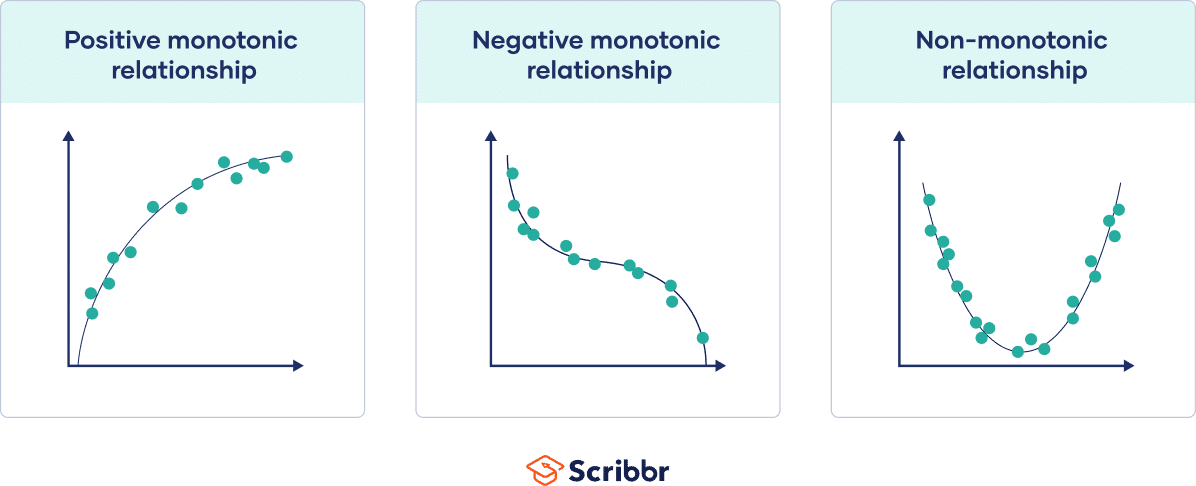
While the Pearson correlation coefficient measures the linearity of relationships, the Spearman correlation coefficient measures the monotonicity of relationships.

In a linear relationship, each variable changes in one direction at the same rate throughout the data range. In a monotonic relationship, each variable also always changes in only one direction but not necessarily at the same rate.

• Positive monotonic: when one variable increases, the other also increases.
• Negative monotonic: when one variable increases, the other decreases.

Monotonic relationships are less restrictive than linear relationships.

 

 Spearman’s rank correlation coefficient formula

The symbols for Spearman’s rho are ρ for the population coefficient and rs for the sample coefficient. The formula calculates the Pearson’s r correlation coefficient between the rankings of the variable data.

To use this formula, you’ll first rank the data from each variable separately from low to high: every datapoint gets a rank from first, second, or third, etc.

Then, you’ll find the differences (di) between the ranks of your variables for each data pair and take that as the main input for the formula.

Spearman’s rank correlation coefficient formula	Explanation
	rs= strength of the rank correlation between variables di = the difference between the x-variable rank and the y-variable rank for each pair of data ∑d2i = sum of the squared differences between x- and y-variable ranks n = sample size

If you have a correlation coefficient of 1, all of the rankings for each variable match up for every data pair. If you have a correlation coefficient of -1, the rankings for one variable are the exact opposite of the ranking of the other variable. A correlation coefficient near zero means that there’s no monotonic relationship between the variable rankings.

Other coefficients

The correlation coefficient is related to two other coefficients, and these give you more information about the relationship between variables.

Coefficient of determination

When you square the correlation coefficient, you end up with the correlation of determination (r2). This is the proportion of common variance between the variables. The coefficient of determination is always between 0 and 1, and it’s often expressed as a percentage.

Coefficient of determination	Explanation
r2	The correlation coefficient multiplied by itself

The coefficient of determination is used in regression models to measure how much of the variance of one variable is explained by the variance of the other variable.

A regression analysis helps you find the equation for the line of best fit, and you can use it to predict the value of one variable given the value for the other variable.

A high r2 means that a large amount of variability in one variable is determined by its relationship to the other variable. A low r2 means that only a small portion of the variability of one variable is explained by its relationship to the other variable; relationships with other variables are more likely to account for the variance in the variable.

The correlation coefficient can often overestimate the relationship between variables, especially in small samples, so the coefficient of determination is often a better indicator of the relationship.

Coefficient of alienation

When you take away the coefficient of determination from unity (one), you’ll get the coefficient of alienation. This is the proportion of common variance not shared between the variables, the unexplained variance between the variables.

Coefficient of alienation	Explanation
1 – r2	One minus the coefficient of determination

A high coefficient of alienation indicates that the two variables share very little variance in common. A low coefficient of alienation means that a large amount of variance is accounted for by the relationship between the variables.

There are several types of correlation coefficients, each suited to analyze different relationships between variables. Here are two common types you might encounter in civil engineering, along with a worked example for each:

Disclaimer: Compiled from different web Resources: